Tag Archives: code

Creating a searchable and sortable list of draft-eligible CHL players using Python and AngularJS

Looking at past NHL Entry Drafts it can be found that a large number of players selected in this event come from the Canadian Hockey League (CHL), namely its three constituents: the Quebec Major Junior Hockey League (QMJHL), the Ontario Hockey League (OHL), and the Western Hockey League (WHL). A quick analysis of the last six drafts shows that a portion of more than 46% of the selected individuals had at that time been playing in on of the three major junior leagues. Even though this percentage used to be higher as other areas and leagues have become and are becoming more important providers of NHL talent, it is safe to assume that this situation won’t change in the foreseeable future.

For the devoted fan of an NHL team this is one additional reason to follow the CHL more closely. Something that – if you’re not able to attend games personally – has become more feasible with the online dissemination of game scores and player statistics. Yet while it is possible to regularly visit each league’s website to retrieve this information, I have found it unexpectedly hard to keep track of which players have already been drafted by an NHL team (as it is very common that these return to junior for one or more seasons) or are still too young to be selected in the upcoming draft. As I am not aware of any list that compiles all candidates that are eligible for the upcoming NHL Entry Draft I have decided to create such a list by myself. The result is already available, however I will try to outline my work to achieve it in the lines below.

Technologically the process introduced consists of two individual operations:

  1. On the back end we have to retrieve the data from the aforementioned websites according to a number of criteria and finally create a suitable compilation containing all desired players and accompanying information. In the example presented here we have a Python script implementation providing the collected data in a JSON file.
  2. On the front end we want to provide means for searching and sorting the compiled data presented on a corresponding website of our own. This is done using the AngularJS framework which enhances regular HTML for dynamic content display.

Back end data retrieval

Let’s start by having a look at the back end. The general workflow for the data retrieval is made up of three working steps. First we are going to retrieve a list of all teams playing in each of the concerned leagues. For each team we will then fetch roster information, i.e. all players associated with the given team. By doing so we are going to register basic information about each player, i.e. height, weight or position but also age and NHL draft status allowing for the sole selection of draft-eligible individuals. In a last step we will then retrieve up-to-date player statistics to be finally represented in the compiled list which itself will a made available as a JSON file.

The complete process is implemented in a Python script that has been made available in the Portolan GitHub repository. Here we are going to shed light on a few selected aspects of it.

To temporarily hold information I have learned to appreciate named tuples as they have been introduced in Python’s collection module with version 2.6. If you don’t need the flexibility and mutability of real objects but still want to have your data well structured and easily accessible, named tuples should be your first choice. Following are the definitions that have been made to keep information about teams, players and player statistics:

from collections import namedtuple

# definition of named tuples to hold some data
# team information
Team = namedtuple('Team', 'id name city code')
# player information
Player = namedtuple('Player', 'id first_name last_name team league 
                               dob draft_day_age is_overager position
                               height weight shoots url')
# single season player statistics
Statline = namedtuple('Statline', 'id season
                                   games_played assists points plus_minus penalty_minutes
                                   power_play_goals power_play_assists power_play_points
                                   short_handed_goals short_handed_assists short_handed_points
                                   shots shooting_percentage points_per_game')

The main criterion to differentiate between players that are draft-eligible and those that are not is age. The exact rule is laid out in the NHL’s Hockey Operation Guidelines, for the upcoming draft it boils down to the following concrete dates (note that the cutoff date does not correspond with the draft date itself hence the separate definition):

from dateutil.parser import parse

# defining dates
# lower date of birth for draft-eligible players, older players do not need to be drafted
LOWER_CUTOFF_DOB = parse("Jan 1, 1997").date()
# regular cutoff date of birth for draft-eligible players, younger ones weren't draft-eligible in the previous draft
REGULAR_CUTOFF_DOB = parse("Sep 15, 1998").date()
# upper cutoff date of birth for draft-eligible players, younger ones are only draft-eligible in the next draft
UPPER_CUTOFF_DOB = parse("Sep 15, 1999").date()
# date of the upcoming draft
DRAFT_DATE = parse("Jun 23, 2017").date()

(Obviously, I am a friend of the dateutil module and you should be, too.)

As with a lot of current websites, the ones of the three leagues in question don’t have their data presently available in regular HTML directives anymore but in associated data streams usually formatted in JSON notation. In our case this holds true for team overviews, roster summaries and even team player statistics. Whilst it is somewhat awkward to find these links in the first place, it is actually quite awesome for scraping as the data is already well-structured and therefore easily accessible. Hence we’re defining look up dictionaries for each league and dataset type (see source code for actual values):

# league-specific template urls for team overview pages
TEAM_OVERVIEW_URLS = {
    'QMJHL': "http://cluster.leaguestat.com/feed/...",
    'OHL': "...",
    'WHL': "...",
}

# league-specific template urls for team roster pages
TEAM_ROSTER_URLS = {
    'QMJHL': "...",
    'OHL': "...",
    'WHL': "...",
}

# league-specific template urls for team statistic pages
TEAM_STATS_URLS = {
    'QMJHL': "...",
    'OHL': "...",
    'WHL': "...",
}

The retrieval itself is actually quite straightforward and follows the workflow outlined above:

if __name__ == '__main__':

    tgt_path = r"junior.json"

    # setting up result containers for rosters and player stats
    full_rosters = dict()
    full_stats = dict()
    
    # doing the following for each league
    for league in ['QMJHL', 'OHL', 'WHL']:
        # retrieving teams in current league
        teams = retrieve_teams(league)
        for team in teams.values()[:]:
            # retrieving roster for current team
            roster = retrieve_roster(team, league)
            # updating container for all rosters
            full_rosters.update(roster)
            # retrieving player statistics for current team
            stats = retrieve_stats(team, league, roster)
            # updating container for all player statistics
            full_stats.update(stats)

    # dumping rosters and stats to JSON file
    dump_to_json_file(tgt_path, full_roster, full_stats)

For implementation of the used functions again see the actual source code over at GitHub.

Finally we have a JSON file with all draft-eligible skaters from the major junior leagues looking like this:

[
..., 
  {
    "assists": 1, 
    "dob": "1999-01-05", 
    "draft_day_age": 18.174, 
    "first_name": "Cole", 
    "games_played": 16, 
    "goals": 1, 
    "height": 6.02, 
    "id": "14853", 
    "is_overager": false, 
    "last_name": "Rafuse", 
    "league": "QMJHL", 
    "penalty_minutes": 2, 
    "plus_minus": 2, 
    "points": 2, 
    "points_per_game": 0.13, 
    "position": "LW", 
    "power_play_assists": 0, 
    "power_play_goals": 0, 
    "power_play_points": 0, 
    "season": "", 
    "shooting_percentage": 11.1, 
    "shoots": "L", 
    "short_handed_assists": 0, 
    "short_handed_goals": 0, 
    "short_handed_points": 0, 
    "shots": 9, 
    "team": [
      2, 
      "Acadie-Bathurst Titan", 
      "Acadie-Bathurst", 
      "Bat"
    ], 
    "url": "http://theqmjhl.ca/players/14853", 
    "weight": "205"
  }, 
...
]

Please note the selected lines that show the actual age of the player on draft day and a boolean variable indicating whether the current player is considered an overager, i.e. could have already been drafted in the previous draft.

Front end data display

The collected data can now be displayed in tabular form. Whilst using regular HTML is perfectly viable to achieve this task, the user can easily be enabled to search, filter and sort the data comfortably by utilizing AngularJS, a JavaScript framework that extends traditional HTML to allow for dynamic information display. Angular builds on the model-view-controller architecture – and it’s not my business to introduce here what has been explained much better somewhere else (for example at the Chrome Developer Page). An important feature of Angular are directives, basically additional HTML attributes that extend the behavior of the corresponding tag. Theses directives usually can be easily recognized as they are starting with the prefix ‘ng-‘. Always striving to create valid HTML I will further add ‘data-‘ to the directive as described as best practice in the AngularJS docs. Otherwise being fairly new to Angular, I have based my work on an example presented at scotch.io.

The solution I have come up with consists of three parts:

  1. An HTML page outlining the basic layout of our page (junior.html).
  2. A JavaScript file containing the logic of our solution (junior.js).
  3. The actual data – this is the JSON file that has been produced by the back end (junior.json).

A very basic version of junior.js could look like the following snippet. We just create an application called showSortJuniorApp and define the main controller. Within this controller there is just one function. It reads the JSON data file and saves its contents within the scope.

angular.module('showSortJuniorApp', [])

.controller('mainController', function($scope, $http) {

  // loading stats from external json file
  $http.get('junior.json').then(function(res) {
      $scope.last_modified = res.data[0]['last_modified'];
      $scope.stats = res.data.slice(1);
  });

});

Now let’s have a look at a basic version of the accompanying junior.html. After importing CSS definitions from Bootstrap and the AngularJS source from Google, we finally include our very own JavaScript file. In the body part (among a few other things) a container element is linked with the app we created above (using the ng-app and ng-controller directives) and a table is defined and populated via the ng-repeat directive. The latter basically provides a loop over the array we loaded in our junior.js and creates a new table row for each element.

<!DOCTYPE html>
<html lang="en">
<head>
    <meta charset="utf-8" />
    <title>Draft-eligible players from QMJHL, OHL and WHL: Summary</title>

    <!-- css -->
    <link rel="stylesheet" href="http://maxcdn.bootstrapcdn.com/bootswatch/3.2.0/spacelab/bootstrap.min.css">
    <style>
        body { padding-top: 40px; }
    </style>

    <!-- javascript -->
    <script type="text/javascript" src="http://ajax.googleapis.com/ajax/libs/angularjs/1.5.8/angular.min.js"></script>
    <script type="text/javascript" src="junior.js"></script>

</head>
<body>
<div class="container" data-ng-app="showSortJuniorApp" data-ng-controller="mainController">
  
  <h1>Skaters from Major Junior Eligible for the 2017 NHL Entry Draft</h1>

  <hr />

  <div class="alert alert-info">
    <p>The following sortable and searchable table contains all skaters from QMJHL, OHL and WHL that are eligible for the 2017 NHL Entry Draft. For a description of the workflow and a detailed explanation of the methodology refer to this <b><a href="http://portolan.leaffan.net/creating-a-searchable-and-sortable-list-of-draft-eligible-chl-players-using-python-and-angularjs/">post</a></b> on the <b><a href="http://portolan.leaffan.net/">Portolan Blog</a></b>.</p>
    <p><b>Last modified:</b> {{ last_modified }}</p>
  </div>

  <table class="table table-bordered table-striped">
     <thead>
         <tr>
             <td>Name</td>
             <td>Team</td>
             <td>Draft Day Age</td>
             <td>GP</td> 
             <td>G</td> 
             <td>A</td> 
             <td>Pts.</td> 
             <td>SH</td> 
             <td>S%</td> 
             <td>P/G</td> 
         </tr>
     </thead>
     <tbody>
         <tr data-ng-repeat="stat in stats">
             <td class="col-md-2"><a data-ng-href="{{ stat.url }}">{{ stat.first_name }} {{ stat.last_name }}</a></td>
             <td class="col-md-2">{{ stat.team[2] }}</td>
             <td class="col-md-1">{{ stat.draft_day_age.toFixed(3) }}</td>
             <td class="col-md-1">{{ stat.games_played }}</td>
             <td class="col-md-1">{{ stat.goals }}</td>
             <td class="col-md-1">{{ stat.assists }}</td>
             <td class="col-md-1">{{ stat.points }}</td>
             <td class="col-md-1">{{ stat.shots }}</td>
             <td class="col-md-1">{{ stat.shooting_percentage.toFixed(1) }}</td>
             <td class="col-md-1">{{ stat.points_per_game.toFixed(2) }}</td>
         </tr>
     </tbody>
</table>

</div>
</body>
</html>

Now how to allow for sortable columns? This can be achieved quite easy. First we define a default sort criterion and order in junior.js:

$scope.statsSortCriterion = 'points'; // default sort criterion
$scope.statsSortDescending = true;    // descending as default sort order

We may then modify the ng-repeat directive in junior.html to make the whole table sort by points in descending order as the default configuration:

<tr data-ng-repeat="stat in stats | orderBy:statsSortCriterion:statsSortDescending">

To create clickable column headings allowing for varying sort criteria an according HTML tag and the ng-click directive have to be added to each header cell of the table in junior.html:

<td>
     <a href="#" data-ng-click="statsSortCriterion = 'draft_day_age'; statsSortDescending = !statsSortDescending">Draft Day Age 
     </a>
</td>
<td>
     <a href="#" data-ng-click="statsSortCriterion = 'games_played'; statsSortDescending = true">GP 
     </a>
</td>

Here we set a descending sort order on the games played column. However to allow for sorting in both directions we can set the variable to take on its negated value. See the example for draft day age above. This configuration will change the sort order every time we click on the column heading.

Finally we would like a search function allowing for the filtering of last names and a checkbox to hide overagers. To do so we first have to add a suitable form to the HTML:

<form>
    <div class="form-group">
        <div class="input-group">
            <div class="input-group-addon"><i class="fa fa-search"></i></div>
            <input type="text" class="form-control" placeholder="Filter by name" data-ng-model="nameFilter" />
        </div>
        <div class="checkbox">
            <label>
                <input type="checkbox" id="a" data-ng-model="hideOveragers" value="Hide overage players" />Hide overage players
            </label>
        </div>
    </div>
</form>

After adding some variables and a short filter function to junior.js…

$scope.nameFilter = '';               // empty name filter
$scope.hideOveragers = false;         // per default overagers are shown

// hiding overagers if corresponding checkbox is checked
$scope.overageFilterFunc = function(a) {
    if ($scope.hideOveragers && a.is_overager) {
      return false;
    } else {
      return true;
    }
};

… we can complete the ng-repeat directive for our tabular data in the following manner:

<tr data-ng-repeat="stat in stats | orderBy:statsSortCriterion:statsSortDescending | filter:nameFilter | filter:overageFilterFunc">

After a few more modifications to the HTML and the JavaScript code, the final version of our front end data display also includes the ability to switch table contents between basic statistics (as used above), player information (such as height, weight, etc.) and additional information (i.e. special team stats). You may refer to the GitHub repository to review the most recent version of this solution.

Speeding up an ArcPy script using the Python multiprocessing module

ArcPy is ESRI’s interface to scripted geoprocessing capabilities. While I personally am much more inclined to use the open-source tool stack of OGR/GDAL, I am stuck with ESRI, ArcGIS and ArcPy at my current professional position. One of my more recent projects presented the need of analyzing a number of point features with regard to nearby line features. In detail the line feature with the smallest distance to the point feature had to be retrieved.

A corresponding algorithm could look like this:

  1. Select a point feature.
  2. Create a buffer around the feature using a base size.
  3. Collect all line features that are situated within the selected buffer.
  4. If no line features were found continually increase buffer size and repeat step 3 until one or more line features have been found.
  5. From the collected line features identify the one with the smallest distance to the selected point feature.

The implementation of this process is straightforward.

#!/usr/bin/env python
import os, sys
import arcpy

sde_connection_file = "sde_connection.sde"

point_src_dataset = "FDS_POINT"
point_src_featureclass = "FCL_POINT"

line_src_dataset = "FDS_LINE"
line_src_featureclass = "FCL_LINE"

buffer_base_increment = 10

point_lyr_src = '\\'.join((sde_connection_file, point_src_dataset, point_src_featureclass))
line_lyr_src = '\\'.join((sde_connection_file, line_src_dataset, line_src_featureclass))


def find_nearest_line(point_lyr_src, line_lyr_src):
    # creating ESRI feature layers
    point_lyr = arcpy.management.MakeFeatureLayer(point_lyr_src, "point_layer")
    line_lyr = arcpy.management.MakeFeatureLayer(line_lyr_src, "line_layer")

    # retrieving OID and shape field names for point feature layer
    oid_fieldname = arcpy.Describe(point_lyr).OIDFieldName
    shape_fieldname = arcpy.Describe(point_lyr).shapeFieldName

    # setting up container for resulting pairs of points and least-distance lines
    pnt_min_dist_line_pairs = list()
    
    with arcpy.da.SearchCursor(point_lyr, ["OID@", "SHAPE@"]) as point_cursor:
        for poid, geom in point_cursor:
            print "Working on point feature %d" % poid
            # setting up a where clause to create a feature layer that solely contains the current point of interest
            poi_where_clause = "%s = %d" % (oid_fieldname, poid)
            # crreating that feature layer that will be used as foundation for distance calculation
            poi_lyr = arcpy.management.MakeFeatureLayer(point_lyr, "poi_layer", poi_where_clause)
    
            buffer_radius = 0
            nearby_lines_cnt = 0
            i = 1
            
            while not nearby_lines_cnt:
                # setting initial buffer radius to base size or incrementing
                # current buffer radius by base size (non-linear)
                buffer_radius += i * buffer_base_increment
                # finding all line elements that are within a distance of
                # buffer radius from the point of interest
                nearby_lines_lyr = arcpy.management.SelectLayerByLocation(line_lyr, "WITHIN_A_DISTANCE", poi_lyr, buffer_radius)
                nearby_lines_cnt = int(arcpy.management.GetCount(nearby_lines_lyr).getOutput(0))
                i += 1

            print "Number of line features found within %d m of point feature %d: %d" % (buffer_radius, poid, nearby_lines_cnt)
            
            # retrieving point geometry
            point_geom = arcpy.PointGeometry(geom.getPart())
    
            # setting up minimal distance variables
            minimal_distance = sys.maxsize
            minimal_distance_line_oid = None
    
            # from all found lines within buffer radius find the one with the
            # smallest distance to the point of interest feature
            with arcpy.da.SearchCursor(nearby_lines_lyr, ["OID@", "SHAPE@"]) as line_cursor:
                for loid, lgeom in line_cursor:
                    line_geom = arcpy.Polyline(lgeom.getPart())
                    distance = point_geom.distanceTo(line_geom)
    
                    if distance < minimal_distance:
                        minimal_distance = distance
                        minimal_distance_line_oid = loid

            print "Minimum distance calculated between point feature %d and line feature %d: %0.2f" % (poid, minimal_distance_line_oid, minimal_distance)
            
            arcpy.management.Delete(poi_lyr)

            pnt_min_dist_line_pairs.append((poid, minimal_distance_line_oid, minimal_distance))
                        
            print "++++++++++++++++++++++++++++++++++++++++++++++++++++++++++++"

    return pnt_min_dist_line_pairs

if __name__ == '__main__':
    
    point_with_least_distance_lines = find_nearest_line(point_lyr_src, line_lyr_src)

Problem with this solution is that depending on the number of point objects to analyze it can be painfully inefficient as we linearly process one item at a time. This may not be problematic if the overall count of items is concise, but real-world data tends to be not to. In my case several thousands of objects had to be regarded leading to a processing time of multiple hours. Whilst optimization is something that should not be done prematurely, I regarded this situation definitely as worth looking into in more detail.

A very common approach to optimize a software solution is to split the complete set of tasks into smaller subsets and to process several of those subsets simultaneously. This approach has become particularly viable with the appearance of multi-core hardware that seems predestined to be used in this manner. From a conceptional viewpoint it is necessary that the individual problems do not interfere with each other. This is clearly the case in the described setup as the minimum distance between a point and a number of line feature is obviously independent from another point feature.

Regarding the point features at hand we will create subsets by splitting the complete dataset into parts that are not larger than a certain cutoff size. An original question over here presents a solution that is already feasible for my demands:

def chunks(l, n):
    u"""
    Yields successive n-sized chunks from l with the last chunk containing
    m (< n) elements.
    """
    for i in xrange(0, len(l), n):
        yield l[i : i + n]

This generic function may now be applied to the actual set of input features:

def get_equal_parts(lyr, size):
    u"""
    Creates oid ranges with given maximum size from specified layer.
    """
    print "Creating oid ranges with maximum size %d" % size
    
    all_oids = list()
    
    with arcpy.da.SearchCursor(lyr, ["OID@"]) as cursor:
        for oid, in cursor:
            all_oids.append(oid)
    
    print "%d oids found overall" % len(all_oids)
    equal_parts = list(chunks(sorted(all_oids), size))
    print "%d oid ranges created" % len(equal_parts)
    return equal_parts

if __name__ == '__main__':
    equal_parts = get_equal_parts(point_lyr_src, 20)    

Please note that is not sufficient to simply retrieve minimum and maximum object ids from the presented layer as previous edits or selections may have created gaps between those values. We actually have to collect all available OIDs instead.

Now for Python, the multiprocessing module (among others) comprises several options to implement parallel solutions. One is to setup a pool of worker processes that subsequently are equipped with according tasks. Here we will supply a number of workers the task to retrieve nearest lines to one of the previously created range of point objects. To do so we have to collect all the necessary data first, i.e. sources for point and line layers as well as the range of OIDs:

if __name__ == '__main__':
    mp_func_data = list()
    i = 0
    for eq in equal_parts:
        i += 1
        print "part %2d - lower oid bound: %4d - upper oid bound: %4d - size: %2d" % (i, eq[0], eq[-1], len(eq))
        mp_func_data.append([point_lyr_src, line_lyr_src, eq[0], eq[-1]])

As you can see we have combined all necessary input data for one chunk into a list object before appending it to an overall list containing the input data for all chunks. This is by design as mapping worker processes to functions only allows one argument. That is also we have to adjust the definition of our worker function:

def find_nearest_line(func_data):
    # unpacking provided function data
    point_lyr_src, line_lyr_src, oid_lower_bound, oid_upper_bound = func_data

    # creating ESRI feature layers
    point_lyr = arcpy.management.MakeFeatureLayer(point_lyr_src, "point_layer")
    line_lyr = arcpy.management.MakeFeatureLayer(line_lyr_src, "line_layer")

    # retrieving OID and shape field names for point feature layer
    oid_fieldname = arcpy.Describe(point_lyr).OIDFieldName
    shape_fieldname = arcpy.Describe(point_lyr).shapeFieldName

    # setting up where clause to restrict selection to specified oid range
    where_clause = "%s >= %d AND %s <= %d" % (oid_fieldname, oid_lower_bound, oid_fieldname, oid_upper_bound)
    # re-create point feature layer
    arcpy.management.Delete(point_lyr)
    point_lyr = arcpy.management.MakeFeatureLayer(point_lyr_src, "point_layer", where_clause)

Finally we create a worker pool and assign each worker a task by mapping it to the function for nearest line retrieval and providing it with the necessary input data:

    # setting up pool of four workers
    pool = multiprocessing.Pool(4, None, None, 1)
    # setting up list for all results
    all_results = list()

    # mapping function for nearest line retrieval (with input data) to worker pool
    for worker_results in pool.map(find_nearest_line, mp_func_data):
        all_results.extend(worker_results)

    # closing pool and waiting for each task to be finished
    pool.close()
    pool.join()

The Pool constructor allows for several arguments. One may define an initialization function that each worker will carry out after being created, this function may of course be provided with initialization arguments. Both of these arguments are set to None in the case at hand. More interesting is the last argument which is set to 1. This is the maximum number of tasks that will be processed by a single worker process before it is killed and a new one is spawned. As ArcPy functions are notorious for leaking memory it is especially necessary to keep this number low or we may end up with exceptions due to low memory.

Implementing multiprocessing for my use case has decreased processing time to a quarter of the previous duration. Now it is still in the range of hours but at least considerable less than in the linear version of this program.

We will have a look at how analysis tasks like the one described above may be sped up by applying low-level database queries in a later post on the Portolan Blog.

An NHL hockey database using Python, PostgreSQL and SQLAlchemy (Pt. 1): Teams and Divisions

Being an avid hockey follower and fan of the National Hockey League’s Toronto Maple Leafs for more than twenty years, I have observed the recent surge of approaches to tackle the sport and its peculiarities based on application of analytical methods with great interest. Of course as a foundation of any data analysis there has to be some data first. Preferably in a standardized and suitable environment such as a relational database management system. My very personal endeavors to retrieve, structure, store and analyze hockey-related data will be subject of a larger series of posts that I am starting today. The series title already lays out the scope within this undertaking will be conducted. I will be looking at the National Hockey League as it provides (with all of its shortcomings) the most detailed data available in this regard. Python as programming language, PostgreSQL as database system and SQLAlchemy as SQL and mapping framework connecting both of the formerly mentioned will serve as my technology stack. But let’s get it on already.

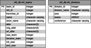
As first part of this series I will be looking at NHL teams and divisions. This is fitting for the beginning as the accompanying data is not very complex and particularly static as well, i.e. it changes with very low frequency. We may provide a simple database entity, i.e. table, containing basic team data using the following SQL data definition statement:

CREATE TABLE nhl_db.nhl_teams
(
  team_id serial NOT NULL,
  nhl_id integer, -- Team id as used on the NHL website
  franchise_id integer, -- Franchise id as used on the NHL website
  name character varying NOT NULL,
  short_name character varying NOT NULL, -- Team nick name
  abbr character(3) NOT NULL,
  orig_abbr character(3) NOT NULL, -- Team abbreviation as used in official game documents on the NHL website
  url_abbr character(3), -- Team abbreviation as previously used in urls on the NHL website
  was_team integer,
  became_team integer,
  init_year integer,
  end_year integer,
  CONSTRAINT nhl_team_key PRIMARY KEY (team_id)
)

As you can see this table design accounts for the fact that from time to time franchises move around or change their names. In case a certain team is the current reincarnation of a given franchise, both became_team and end_year contain NULL values thus marking it as active.

To whom it may concern: Differentiating between the various abbreviation types is necessary due to the NHL using different ways of shorting a team name on game reports (N.J, L.A,…) and in URLs (NJD, LAK,…). Additionally I wasn’t happy with some of their choices for abbreviations so that I created my very own column.

Update (February 2016): With the current update of the NHL’s website the previous system of using abbreviations for team identification was abolished and actual team (and franchise) ids have been introduced. The according changes in the data model are marked above. As far as I have grasped the url_abbr column should no longer be necessary, I will keep it for safety and nostalgic reasons though.

After setting up the table data insertion may be conducted easily by preparing and applying the according SQL insert statements. Both nhl_id and franchise_id values have been retrieved from the NHL’s website.

INSERT INTO nhl_db.nhl_teams (team_id, name, short_name, abbr, orig_abbr, url_abbr, was_team, became_team, init_year, end_year, nhl_id, franchise_id) VALUES (0, 'Anaheim Ducks', 'Ducks', 'ANA', 'ANA', 'ANA', 38, NULL, 2006, NULL, 24, 32);
INSERT INTO nhl_db.nhl_teams (team_id, name, short_name, abbr, orig_abbr, url_abbr, was_team, became_team, init_year, end_year, nhl_id, franchise_id) VALUES (1, 'Boston Bruins', 'Bruins', 'BOS', 'BOS', 'BOS', NULL, NULL, 1924, NULL, 6, 6);
INSERT INTO nhl_db.nhl_teams (team_id, name, short_name, abbr, orig_abbr, url_abbr, was_team, became_team, init_year, end_year, nhl_id, franchise_id) VALUES (2, 'Buffalo Sabres', 'Sabres', 'BUF', 'BUF', 'BUF', NULL, NULL, 1970, NULL, 7, 19);
INSERT INTO nhl_db.nhl_teams (team_id, name, short_name, abbr, orig_abbr, url_abbr, was_team, became_team, init_year, end_year, nhl_id, franchise_id) VALUES (3, 'Calgary Flames', 'Flames', 'CGY', 'CGY', 'CGY', 31, NULL, 1980, NULL, 20, 21);
INSERT INTO nhl_db.nhl_teams (team_id, name, short_name, abbr, orig_abbr, url_abbr, was_team, became_team, init_year, end_year, nhl_id, franchise_id) VALUES (4, 'Carolina Hurricanes', 'Hurricanes', 'CAR', 'CAR', 'CAR', 32, NULL, 1997, NULL, 12, 26);
INSERT INTO nhl_db.nhl_teams (team_id, name, short_name, abbr, orig_abbr, url_abbr, was_team, became_team, init_year, end_year, nhl_id, franchise_id) VALUES (5, 'Chicago Blackhawks', 'Blackhawks', 'CHI', 'CHI', 'CHI', 43, NULL, 1986, NULL, 16, 11);
INSERT INTO nhl_db.nhl_teams (team_id, name, short_name, abbr, orig_abbr, url_abbr, was_team, became_team, init_year, end_year, nhl_id, franchise_id) VALUES (6, 'Colorado Avalanche', 'Avalanche', 'COL', 'COL', 'COL', 33, NULL, 1995, NULL, 21, 27);
INSERT INTO nhl_db.nhl_teams (team_id, name, short_name, abbr, orig_abbr, url_abbr, was_team, became_team, init_year, end_year, nhl_id, franchise_id) VALUES (7, 'Columbus Blue Jackets', 'Blue Jackets', 'CLB', 'CBJ', 'CBJ', NULL, NULL, 2000, NULL, 29, 36);
INSERT INTO nhl_db.nhl_teams (team_id, name, short_name, abbr, orig_abbr, url_abbr, was_team, became_team, init_year, end_year, nhl_id, franchise_id) VALUES (8, 'Dallas Stars', 'Stars', 'DAL', 'DAL', 'DAL', 34, NULL, 1993, NULL, 25, 15);
INSERT INTO nhl_db.nhl_teams (team_id, name, short_name, abbr, orig_abbr, url_abbr, was_team, became_team, init_year, end_year, nhl_id, franchise_id) VALUES (9, 'Detroit Red Wings', 'Red Wings', 'DET', 'DET', 'DET', NULL, NULL, 1926, NULL, 17, 12);
INSERT INTO nhl_db.nhl_teams (team_id, name, short_name, abbr, orig_abbr, url_abbr, was_team, became_team, init_year, end_year, nhl_id, franchise_id) VALUES (10, 'Edmonton Oilers', 'Oilers', 'EDM', 'EDM', 'EDM', NULL, NULL, 1979, NULL, 22, 25);
INSERT INTO nhl_db.nhl_teams (team_id, name, short_name, abbr, orig_abbr, url_abbr, was_team, became_team, init_year, end_year, nhl_id, franchise_id) VALUES (11, 'Florida Panthers', 'Panthers', 'FLA', 'FLA', 'FLA', NULL, NULL, 1993, NULL, 13, 33);
INSERT INTO nhl_db.nhl_teams (team_id, name, short_name, abbr, orig_abbr, url_abbr, was_team, became_team, init_year, end_year, nhl_id, franchise_id) VALUES (12, 'Los Angeles Kings', 'Kings', 'LAK', 'L.A', 'LAK', NULL, NULL, 1967, NULL, 26, 14);
INSERT INTO nhl_db.nhl_teams (team_id, name, short_name, abbr, orig_abbr, url_abbr, was_team, became_team, init_year, end_year, nhl_id, franchise_id) VALUES (13, 'Minnesota Wild', 'Wild', 'MIN', 'MIN', 'MIN', NULL, NULL, 2000, NULL, 30, 37);
INSERT INTO nhl_db.nhl_teams (team_id, name, short_name, abbr, orig_abbr, url_abbr, was_team, became_team, init_year, end_year, nhl_id, franchise_id) VALUES (14, 'Montreal Canadiens', 'Canadiens', 'MTL', 'MTL', 'MTL', NULL, NULL, 1917, NULL, 8, 1);
INSERT INTO nhl_db.nhl_teams (team_id, name, short_name, abbr, orig_abbr, url_abbr, was_team, became_team, init_year, end_year, nhl_id, franchise_id) VALUES (15, 'Nashville Predators', 'Predators', 'NSH', 'NSH', 'NSH', NULL, NULL, 1998, NULL, 18, 34);
INSERT INTO nhl_db.nhl_teams (team_id, name, short_name, abbr, orig_abbr, url_abbr, was_team, became_team, init_year, end_year, nhl_id, franchise_id) VALUES (16, 'New Jersey Devils', 'Devils', 'NJD', 'N.J', 'NJD', 35, NULL, 1982, NULL, 1, 23);
INSERT INTO nhl_db.nhl_teams (team_id, name, short_name, abbr, orig_abbr, url_abbr, was_team, became_team, init_year, end_year, nhl_id, franchise_id) VALUES (17, 'New York Islanders', 'Islanders', 'NYI', 'NYI', 'NYI', NULL, NULL, 1972, NULL, 2, 22);
INSERT INTO nhl_db.nhl_teams (team_id, name, short_name, abbr, orig_abbr, url_abbr, was_team, became_team, init_year, end_year, nhl_id, franchise_id) VALUES (18, 'New York Rangers', 'Rangers', 'NYR', 'NYR', 'NYR', NULL, NULL, 1926, NULL, 3, 10);
INSERT INTO nhl_db.nhl_teams (team_id, name, short_name, abbr, orig_abbr, url_abbr, was_team, became_team, init_year, end_year, nhl_id, franchise_id) VALUES (19, 'Ottawa Senators', 'Senators', 'OTW', 'OTT', 'OTT', NULL, NULL, 1992, NULL, 9, 30);
INSERT INTO nhl_db.nhl_teams (team_id, name, short_name, abbr, orig_abbr, url_abbr, was_team, became_team, init_year, end_year, nhl_id, franchise_id) VALUES (20, 'Philadelphia Flyers', 'Flyers', 'PHI', 'PHI', 'PHI', NULL, NULL, 1967, NULL, 4, 16);
INSERT INTO nhl_db.nhl_teams (team_id, name, short_name, abbr, orig_abbr, url_abbr, was_team, became_team, init_year, end_year, nhl_id, franchise_id) VALUES (21, 'Phoenix Coyotes', 'Coyotes', 'PHO', 'PHX', 'PHX', 36, 44, 1996, 2014, 27, 28);
INSERT INTO nhl_db.nhl_teams (team_id, name, short_name, abbr, orig_abbr, url_abbr, was_team, became_team, init_year, end_year, nhl_id, franchise_id) VALUES (22, 'Pittsburgh Penguins', 'Penguins', 'PIT', 'PIT', 'PIT', NULL, NULL, 1967, NULL, 5, 17);
INSERT INTO nhl_db.nhl_teams (team_id, name, short_name, abbr, orig_abbr, url_abbr, was_team, became_team, init_year, end_year, nhl_id, franchise_id) VALUES (23, 'San Jose Sharks', 'Sharks', 'SJS', 'S.J', 'SJS', NULL, NULL, 1991, NULL, 28, 29);
INSERT INTO nhl_db.nhl_teams (team_id, name, short_name, abbr, orig_abbr, url_abbr, was_team, became_team, init_year, end_year, nhl_id, franchise_id) VALUES (24, 'St. Louis Blues', 'Blues', 'STL', 'STL', 'STL', NULL, NULL, 1967, NULL, 19, 18);
INSERT INTO nhl_db.nhl_teams (team_id, name, short_name, abbr, orig_abbr, url_abbr, was_team, became_team, init_year, end_year, nhl_id, franchise_id) VALUES (25, 'Tampa Bay Lightning', 'Lightning', 'TBL', 'T.B', 'TBL', NULL, NULL, 1992, NULL, 14, 31);
INSERT INTO nhl_db.nhl_teams (team_id, name, short_name, abbr, orig_abbr, url_abbr, was_team, became_team, init_year, end_year, nhl_id, franchise_id) VALUES (26, 'Toronto Maple Leafs', 'Maple Leafs', 'TOR', 'TOR', 'TOR', 52, NULL, 1927, NULL, 10, 5);
INSERT INTO nhl_db.nhl_teams (team_id, name, short_name, abbr, orig_abbr, url_abbr, was_team, became_team, init_year, end_year, nhl_id, franchise_id) VALUES (27, 'Vancouver Canucks', 'Canucks', 'VAN', 'VAN', 'VAN', NULL, NULL, 1970, NULL, 23, 20);
INSERT INTO nhl_db.nhl_teams (team_id, name, short_name, abbr, orig_abbr, url_abbr, was_team, became_team, init_year, end_year, nhl_id, franchise_id) VALUES (28, 'Washington Capitals', 'Capitals', 'WSH', 'WSH', 'WSH', NULL, NULL, 1974, NULL, 15, 24);
INSERT INTO nhl_db.nhl_teams (team_id, name, short_name, abbr, orig_abbr, url_abbr, was_team, became_team, init_year, end_year, nhl_id, franchise_id) VALUES (29, 'Winnipeg Jets', 'Jets', 'WPG', 'WPG', 'WPG', 30, NULL, 2011, NULL, 52, 35);
INSERT INTO nhl_db.nhl_teams (team_id, name, short_name, abbr, orig_abbr, url_abbr, was_team, became_team, init_year, end_year, nhl_id, franchise_id) VALUES (30, 'Atlanta Thrashers', 'Thrashers', 'ATL', 'ATL', 'ATL', NULL, 29, 1999, 2011, 11, 35);
INSERT INTO nhl_db.nhl_teams (team_id, name, short_name, abbr, orig_abbr, url_abbr, was_team, became_team, init_year, end_year, nhl_id, franchise_id) VALUES (31, 'Atlanta Flames', 'Flames', 'ATF', 'AFM', NULL, NULL, 3, 1972, 1980, 47, 21);
INSERT INTO nhl_db.nhl_teams (team_id, name, short_name, abbr, orig_abbr, url_abbr, was_team, became_team, init_year, end_year, nhl_id, franchise_id) VALUES (32, 'Hartford Whalers', 'Whalers', 'HFD', 'HFD', 'HFD', NULL, 4, 1979, 1997, 34, 26);
INSERT INTO nhl_db.nhl_teams (team_id, name, short_name, abbr, orig_abbr, url_abbr, was_team, became_team, init_year, end_year, nhl_id, franchise_id) VALUES (33, 'Quebec Nordiques', 'Nordiques', 'QUE', 'QUE', 'QUE', NULL, 6, 1979, 1995, 32, 27);
INSERT INTO nhl_db.nhl_teams (team_id, name, short_name, abbr, orig_abbr, url_abbr, was_team, became_team, init_year, end_year, nhl_id, franchise_id) VALUES (34, 'Minnesota North Stars', 'North Stars', 'MNS', 'MNS', 'MNS', NULL, 8, 1967, 1993, 31, 15);
INSERT INTO nhl_db.nhl_teams (team_id, name, short_name, abbr, orig_abbr, url_abbr, was_team, became_team, init_year, end_year, nhl_id, franchise_id) VALUES (35, 'Colorado Rockies', 'Rockies', 'CLR', 'CLR', NULL, 37, 16, 1976, 1982, 35, 23);
INSERT INTO nhl_db.nhl_teams (team_id, name, short_name, abbr, orig_abbr, url_abbr, was_team, became_team, init_year, end_year, nhl_id, franchise_id) VALUES (36, 'Winnipeg Jets', 'Jets', 'WIN', 'WIN', 'WIN', NULL, 21, 1979, 1996, 33, 28);
INSERT INTO nhl_db.nhl_teams (team_id, name, short_name, abbr, orig_abbr, url_abbr, was_team, became_team, init_year, end_year, nhl_id, franchise_id) VALUES (37, 'Kansas City Scouts', 'Scouts', 'KCS', 'KCS', NULL, NULL, 35, 1974, 1976, 48, 23);
INSERT INTO nhl_db.nhl_teams (team_id, name, short_name, abbr, orig_abbr, url_abbr, was_team, became_team, init_year, end_year, nhl_id, franchise_id) VALUES (38, 'Mighty Ducks of Anaheim', 'Mighty Ducks', 'MDA', 'ANA', NULL, NULL, 0, 1993, 2006, 24, 32);
INSERT INTO nhl_db.nhl_teams (team_id, name, short_name, abbr, orig_abbr, url_abbr, was_team, became_team, init_year, end_year, nhl_id, franchise_id) VALUES (39, 'California Seals', 'Seals', 'CSE', 'CSE', NULL, NULL, 40, 1967, 1967, 56, 13);
INSERT INTO nhl_db.nhl_teams (team_id, name, short_name, abbr, orig_abbr, url_abbr, was_team, became_team, init_year, end_year, nhl_id, franchise_id) VALUES (40, 'Oakland Seals', 'Seals', 'OAK', 'OAK', NULL, 39, 41, 1967, 1970, 46, 13);
INSERT INTO nhl_db.nhl_teams (team_id, name, short_name, abbr, orig_abbr, url_abbr, was_team, became_team, init_year, end_year, nhl_id, franchise_id) VALUES (41, 'California Golden Seals', 'Golden Seals', 'CGS', 'CGS', NULL, 40, 42, 1970, 1976, 46, 13);
INSERT INTO nhl_db.nhl_teams (team_id, name, short_name, abbr, orig_abbr, url_abbr, was_team, became_team, init_year, end_year, nhl_id, franchise_id) VALUES (42, 'Cleveland Barons', 'Barons', 'CBN', 'CBN', NULL, 41, NULL, 1976, 1978, 49, 13);
INSERT INTO nhl_db.nhl_teams (team_id, name, short_name, abbr, orig_abbr, url_abbr, was_team, became_team, init_year, end_year, nhl_id, franchise_id) VALUES (43, 'Chicago Black Hawks', 'Black Hawks', 'CHB', 'CHI', NULL, NULL, 5, 1926, 1986, 16, 11);
INSERT INTO nhl_db.nhl_teams (team_id, name, short_name, abbr, orig_abbr, url_abbr, was_team, became_team, init_year, end_year, nhl_id, franchise_id) VALUES (44, 'Arizona Coyotes', 'Coyotes', 'ARI', 'ARI', 'ARI', 21, NULL, 2014, NULL, 53, 28);
INSERT INTO nhl_db.nhl_teams (team_id, name, short_name, abbr, orig_abbr, url_abbr, was_team, became_team, init_year, end_year, nhl_id, franchise_id) VALUES (45, 'Ottawa Senators (1917)', 'Senators (1917)', 'SEN', 'SEN', NULL, NULL, NULL, 1917, 1935, 36, 3);
INSERT INTO nhl_db.nhl_teams (team_id, name, short_name, abbr, orig_abbr, url_abbr, was_team, became_team, init_year, end_year, nhl_id, franchise_id) VALUES (46, 'Hamilton Tigers', 'Tigers', 'HAM', 'HAM', NULL, NULL, NULL, 1919, 1925, 37, 4);
INSERT INTO nhl_db.nhl_teams (team_id, name, short_name, abbr, orig_abbr, url_abbr, was_team, became_team, init_year, end_year, nhl_id, franchise_id) VALUES (47, 'Montreal Wanderers', 'Wanderers', 'MWN', 'MWN', NULL, NULL, NULL, 1917, 1918, 41, 2);
INSERT INTO nhl_db.nhl_teams (team_id, name, short_name, abbr, orig_abbr, url_abbr, was_team, became_team, init_year, end_year, nhl_id, franchise_id) VALUES (48, 'Montreal Maroons', 'Maroons', 'MMR', 'MMR', NULL, NULL, NULL, 1924, 1938, 43, 7);
INSERT INTO nhl_db.nhl_teams (team_id, name, short_name, abbr, orig_abbr, url_abbr, was_team, became_team, init_year, end_year, nhl_id, franchise_id) VALUES (49, 'New York Americans', 'Americans', 'NYA', 'NYA', NULL, NULL, NULL, 1925, 1942, 44, 8);
INSERT INTO nhl_db.nhl_teams (team_id, name, short_name, abbr, orig_abbr, url_abbr, was_team, became_team, init_year, end_year, nhl_id, franchise_id) VALUES (50, 'Pittsburgh Pirates', 'Pirates', 'PIR', 'PIR', NULL, NULL, NULL, 1925, 1931, 38, 9);
INSERT INTO nhl_db.nhl_teams (team_id, name, short_name, abbr, orig_abbr, url_abbr, was_team, became_team, init_year, end_year, nhl_id, franchise_id) VALUES (51, 'Toronto Arenas', 'Arenas', 'TAN', 'TAN', NULL, NULL, 52, 1918, 1919, 57, 5);
INSERT INTO nhl_db.nhl_teams (team_id, name, short_name, abbr, orig_abbr, url_abbr, was_team, became_team, init_year, end_year, nhl_id, franchise_id) VALUES (52, 'Toronto St. Patricks', 'St. Patricks', 'TSP', 'TSP', NULL, 51, 26, 1919, 1927, 58, 5);

A table containing NHL divisions may be set up using the following definition:

CREATE TABLE nhl_db.nhl_divisions
(
  division_id serial NOT NULL,
  division_name character varying,
  year integer, -- Year in which this division was active.
  teams integer[], -- IDs of team constituting this division.
  conference character varying, -- Name of the Conference this division belongs to.
  CONSTRAINT nhl_division_key PRIMARY KEY (division_id)
)

Here a particular property of PostgreSQL is visible: the ability to store multidimensional arrays of varying length in a database column. In this case the teams column will contain the IDs of the teams that set up a certain division at a certain time. Unfortunately there is currently no support for referential integrity between the elements of an array (here: team_ids in column teams of table nhl_divisions) and the elements of another table (column team_id in table nhl_teams). Although amends have been made to introduce this feature in more than just one of the more recent releases, it hasn’t become part of the code base yet.

We will deal with inserting data into this table later on.

Subsequently an (updated) ERD of the current database configuration looks like the following:

nhl_teams_nhl_divisions_update

Using SQLAlchemy it is now very easy to map these tables to Python classes. While it is very viable to use SQLAlchemy magic to set up the table structures from Python, I personally like to go the other way around: Having tables already defined in the database system and mapping it to Python by metadata reflection. Everything that is necessary to do so is the mapped class being inherited from the SQLAlchemy Base class and it having two special attributes __tablename__ and __autoload__.

# conducting necessary imports
from sqlalchemy import create_engine
from sqlalchemy.orm.session import sessionmaker
from sqlalchemy.schema import MetaData
from sqlalchemy.ext.declarative import declarative_base

from sqlalchemy import or_, and_
from sqlalchemy.sql.expression import func

# setting up database connection information
db_engine = 'postgresql'
user = '***
password = '***'
host = '***
port = '5432'
database = 'nhl_test'

conn_string = "%s://%s:%s@%s:%s/%s" % (db_engine, user, password, host, port, database)

# setting up database connection
Engine = create_engine(conn_string, echo = False, pool_size = 5)
# creating session
Session = sessionmaker(bind = Engine)
# setting up base class
Base = declarative_base(metadata = MetaData(schema = 'nhl_db', bind = Engine))

class NHLTeam(Base):
    u"""A class representing an NHL team.
    """
    __tablename__ = 'nhl_teams' # maps this class to table nhl_teams
    __autoload__ = True # sets up metadata reflection

    def __init__(self):
        pass

    def __str__(self):
        return self.name

We may now add a way to search for team objects in the database, i.e. by implementing according class methods to search the database using an abbreviation or team id. Additionally we will add means to make teams comparable and sortable by using Python’s comparison methods.

    @classmethod
    def find(cls, abbr):
        session = Session()
        try:
            t = session.query(NHLTeam).filter(
                    func.lower(NHLTeam.abbr) == abbr.lower()
                ).one()
        except:
            t = None
        finally:
            session.close()
        return t

    @classmethod
    def find_by_id(cls, team_id):
        session = Session()
        try:
            t = session.query(NHLTeam).filter(
                    NHLTeam.team_id == team_id
                ).one()
        except:
            t = None
        finally:
            session.close()
        return t

    @classmethod
    def find_by_nhl_id(self, nhl_id):
        session = Session()
        try:
            t = session.query(NHLTeam).filter(
                NHLTeam.nhl_id == nhl_id
            ).one()
        except:
            t = None
        finally:
            session.close()
        return t

    def __eq__(self, other):
        return self.name == other.name
    
    def __ne__(self, other):
        return not self == other
    
    def __gt__(self, other):
        return self.name > other.name
    
    def __lt__(self, other):
        return self.name < other.name

Please note that this use of Session is actually not recommended. Instead a scoped session should be your choice in production circumstances. However here the more simple approach has been used here for the sake of clarity.

It is now possible to find an NHLTeam object by specifying its abbreviation:

if __name__ == '__main__':
    t = NHLTeam.find('TOR')
    print "Team by abbreviation '%s': %s" % ('TOR', t)
    t = NHLTeam.find_by_id(12)
    print "Team by id %d: %s" % (12, t)

This gives you:

Team with abbreviation 'TOR': Toronto Maple Leafs
Team with id 12: Los Angeles Kings

Similarly we may map the database table containing NHL Division information with an according Python class. As we're creating division data from Python as well, we're including a real constructor this time:

    class NHLDivision(Base):
    u"""A class representing an NHL division.
    """
    __tablename__ = 'nhl_divisions'
    __autoload__ = True

    def __init__(self, name, season, teams, conference = None):
        self.division_name = name
        self.year = season
        self.teams = list()
        for t in teams:
            self.teams.append(t.team_id)
        self.conference = conference

Given definitions and mappings for both team and division objects and having some source data ready, it is now convenient to insert division data using a special helper method:

def create_divisions(division_src_file):
    lines = open(division_src_file).readlines()
    
    session = Session()
    try:
        for line in lines:
            if line.startswith("#"):
                continue
            division_name, season, teams, conference = line.strip().split(";")
            season = int(season)
            # retrieving team abbreviations from source input line
            team_abbrs = teams[1:-1].split(',')
            teams = list()
            # converting abbreviations into team objects
            for t in team_abbrs:
                team = NHLTeam.find(t)
                teams.append(team)
            else:
                if conference:
                    division = NHLDivision(division_name, season, teams, conference)
                else:
                    division = NHLDivision(division_name, season, teams)
                session.add(division)
                
                ids = "{" + ",".join([str(t.team_id) for t in teams])  + "}"
                if conference:
                    output = "%s Division (%s Conference):\t%d\t%s" % (division_name, conference, season, ids)
                else:
                    output = "%s Division:\t%d\t%s" % (division_name, season, ids)
                print output
        else:
            session.commit()
    except:
        session.rollback()

if __name__ == '__main__':
    create_divisions(r"nhl_division_config.txt")

Now if we finally want to determine the league configuration for a given season we can do so by linking division data and the year in question by providing the NHLDivision object definition with the following class method:

    @classmethod
    def get_divisions_and_teams(cls, year):
        session = Session()
        # finding all divisions for this season
        divs = session.query(NHLDivision).filter(
            NHLDivision.year == year).all()
        # linking divisions and teams
        for d in divs:
            teams = list()
            for team_id in d.teams:
                team = NHLTeam.find_by_id(team_id)
                teams.append(team)
            print "%s Division:" % d.division_name
            for t in teams:
                print "\t", t

if __name__ == '__main__':
    NHLDivision.get_divisions_and_teams(2015)

Accordingly this results in:

Pacific Division:
        Anaheim Ducks
        Arizona Coyotes
        Calgary Flames
        Edmonton Oilers
        Los Angeles Kings
        San Jose Sharks
        Vancouver Canucks
Central Division:
        Chicago Blackhawks
        Colorado Avalanche
        Dallas Stars
        Minnesota Wild
        Nashville Predators
        St. Louis Blues
        Winnipeg Jets
Atlantic Division:
        Boston Bruins
        Buffalo Sabres
        Detroit Red Wings
        Florida Panthers
        Montreal Canadiens
        Ottawa Senators
        Tampa Bay Lightning
        Toronto Maple Leafs
Metropolitan Division:
        Carolina Hurricanes
        Columbus Blue Jackets
        New Jersey Devils
        New York Islanders
        New York Rangers
        Philadelphia Flyers
        Pittsburgh Penguins
        Washington Capitals

Class definitions for both NHLTeam and NHLDivision are available via GitHub. In the next installment of this series we will have a look at the table and class definition for NHL player data.

Creating sample points (Pt. 3): Uniform random sampling – Triangulation

The third edition of this series will introduce a more complex sampling method to create points that are spread both randomly and uniformly over the area of a given source polygon.

Previously published parts of this series include:

Uniform random sampling

To distribute points in a polygon in a uniform and random manner we are going to follow an approach laid out within the scope of a discussion amongst MATLAB users. In case the internet will forget this minor thread someday, here’s the reduction of the problem as laid out by merited forum contributor John D’Errico:

“[…] the general approach […] that generates uniform random points inside a general object in n-dimensions.

“Compute the area/volume of each simplex, then assign points to them randomly with probability defined by their area relative to the total area. Within each simplex, […] use a […] method of generating random points […].

“Of course, you need a triangulation of the polygon, but as long as the polygon is a convex one, this is trivial with [D]elaunay.”

To summarize these are steps necessary to create uniform random points in a polygon:

  1. Use the polygon’s vertices to create a Delaunay triangulation. As we can’t guarantee that real-world data will only contain convex geometries, this needs to be generalized form of it, a constrained Delaunay triangulation.
  2. Use the area of each created triangle to create a weighted random selection, i.e. to assure that larger triangles a picked more likely than smaller ones.
  3. Randomly create a point inside the selected triangle.

Now these procedure shall be repeated until a certain stop criterion is fulfilled, something that we will discuss later on. Let’s start with triangualation first.

Delaunay triangulation and constrained Delaunay triangulation

Whilst the original (C++) OGR library contains a method DelaunayTriangulation to retrieve just that for an input geometry, this function is not part of the OGR Python bindings. However, as with most tasks there is already another library that can do what we want. In this case we refer to poly2tri. Originally provided in Java and C++, there also exists a Python version of it. (There are some peculiar patches necessary to get poly2tri to work under Python that I will devote another blog entry for.)

Using Shapely and poly2tri it is now possible to initiate a constrained Delaunay triangulation (CDT):

>>> # creating a source polygon first
>>> from shapely.geometry import Polygon
>>> from shapely.wkt import loads
>>> polygon = loads(open(r"real_world_data.wkt").read())
>>> # preparing list of vertices and adding those of current polygon to it
>>> vertices = list()
>>> for coord_pair in polygon.exterior.coords:
...     vertices.append(coord_pair)
>>> # p2t is the Python module name for poly2tri
>>> import p2t

Now two things have to be considered. First, poly2tri brings its very own Point definition that needs to be distinguished from the one Shapely provides by explicitly using the prefix p2t. Adding to that it must be avoided that the CDT is fed with duplicate points – i.e. as first and last vertex are usually specified in polygon definition. We can deal with this constraint by omitting the first vertex:

>>> # making sure that only one of first or last vertex
>>> # is used to create list of input points for triangulation
>>> border = [p2t.Point(x, y) for x, y in vertices[1:]]
>>> # setting up constrained Delaunay triangulation
>>> cdt = p2t.CDT(border)

Now real-world data kicks in back again as it may contain holes, or interior rings as they are called correctly. These need to be specified separately as input for the CDT:

>>> for interior_ring in polygon.interiors:
...     hole = list()
...     for coord_pair in interior_ring.coords:
...             hole.append(coord_pair)
...     else:
...             cdt.add_hole([p2t.Point(x, y) for x, y in hole[1:]])

Finally, the triangulation can be performed:

>>> triangulation = cdt.triangulate()
>>> print len(triangulation)
1964
>>> for t in triangulation:
...     triangle = Polygon([(t.a.x, t.a.y), (t.b.x, t.b.y), (t.c.x, t.c.y)])
...     print triangle
...
POLYGON ((366392.3774440361 5640960.820684713, 367546.1057238859 5641233.076879927, 366393.6058517902 5641064.830985503, 366392.3774440361 5640960.820684713))
POLYGON ((366393.6058517902 5641064.830985503, 367546.1057238859 5641233.076879927, 367452.1526190441 5641333.95416048, 366393.6058517902 5641064.830985503))
...
...

Following is the visual result of the triangulation.

A constrained Delaunay triangulation was applied to this real-world polygon.

Next up in line to create uniformly random sample points are weighted random selection of triangles and random generation of points inside such a given triangle.

Creating sample points (Pt. 2): Regular grid sampling

In this edition of our series dedicated to polygon sampling techniques we will look into the process of creating regularly gridded sample points with non-uniform intervals.

Previously published parts of this series include:

Regular grid sampling

Using a single point to represent a whole polygon geometry may satisfy only the most basic sampling demands. Another – and certainly more applicable – way to arrange sample points is to create virtual grids of such points that stretch out over the whole area of the polygon to be processed. To do so we need a regular interval between sample points that may be defined identical (i.e. uniform) in both x- and y-direction. Here we will go the more generic route and implement separately adjustable (i.e. non-uniform) intervals for x and y.

The value range of sample coordinates is of course laid out by the extent of the source polygon. Using Shapely the extent of a polygon is called forth by the property bounds:

>>> from shapely.geometry import Polygon
>>> polygon = Polygon([(0,0), (6,0), (0,6)])
>>> print polygon.bounds
(0.0, 0.0, 6.0, 6.0)

Given two intervals in x and y it is now easy to create points at regular gridded positions laid out over the extent of the source polygon. Additionally it should be assured that created points are actually within the polygon to be sampled.

>>> from shapely.geometry import Point
>>> bounds = polygon.bounds
>>> ll = bounds[:2] # lower left coordinate pair of polygon's extent
>>> ur = bounds[2:] # upper right                  ~
>>> x_interval = 1.5
>>> y_interval = 2.0
>>> for x in floatrange(ll[0], ur[0], x_interval):
...     for y in floatrange(ll[1], ur[1], y_interval):
...             point = Point(x, y)
...             if point.within(polygon):
...                     print point
...
POINT (1.5 2)
POINT (1.5 4)
POINT (3 2)

Now real-world spatial data is different yet again as it rarely comes with extents fitting to full meters. It is still possible to have regularly gridded sample points that have *nicely* looking coordinates by creating extent ceilings and floors used as base for the sampling process. We can actually use our defined intervals to create these values:

>>> from shapely.wkt import loads
>>> polygon = loads(open(r"real_world_data.wkt").read())
>>> polygon.bounds
(366392.3774440361, 5630693.4900143575, 373404.5164361303, 5641855.842006282)
>>> ll = polygon.bounds[:2]
>>> ur = polygon.bounds[2:]
>>> x_interval = 100
>>> y_interval = 200
>>> low_x = int(ll[0]) / x_interval * x_interval
>>> upp_x = int(ur[0]) / x_interval * x_interval + x_interval
>>> low_y = int(ll[1]) / y_interval * y_interval
>>> upp_y = int(ur[1]) / y_interval * y_interval + y_interval
>>> print low_x, upp_x, low_y, upp_y
366300 373500 5630600 5642000

Putting it all together

To extend our previously introduced PolygonPointSampler, we can combine all our findings in a new sub class RegularGridSampler. This one will also make use of the possibility of creating a separate constructor as there is the need to define the sampling intervals.

class RegularGridSampler(PolygonPointSampler):
    def __init__(self, polygon = '', x_interval = 100, y_interval = 100):
        super(self.__class__, self).__init__(polygon)
        self.x_interval = x_interval
        self.y_interval = y_interval
    
    def perform_sampling(self):
        u"""
        Perform sampling by substituting the polygon with a regular grid of
        sample points within it. The distance between the sample points is
        given by x_interval and y_interval.
        """
        if not self.prepared:
            self.prepare_sampling()
        ll = self.polygon.bounds[:2]
        ur = self.polygon.bounds[2:]
        low_x = int(ll[0]) / self.x_interval * self.x_interval
        upp_x = int(ur[0]) / self.x_interval * self.x_interval + self.x_interval
        low_y = int(ll[1]) / self.y_interval * self.y_interval
        upp_y = int(ur[1]) / self.y_interval * self.y_interval + self.y_interval
        
        for x in floatrange(low_x, upp_x, self.x_interval):
            for y in floatrange(low_y, upp_y, self.y_interval):
                p = Point(x, y)
                if p.within(self.polygon):
                    self.samples.append(p)

Using our real-world example and a (uniform) sampling interval of 1,000 meters we arrive at the following result:

A real-world polygon with a regular grid of sampling points.

We may also use non-uniform sampling intervals of 1,000 meters in x- and 500 meters in y-direction:

A real-world polygon with a regular grid of sampling points using non-uniform sampling intervals.

A multi-part polygon may also be used to apply the sampler, for example with a uniform sampling interval of 250 m:

A multi-part polygon consisting of four parts sampled by a regular grid with a uniform sampling interval of 250 m.

WTH is a floatrange?

In the meantime you most likely have already realized that we’re using a non-standard range function to iterate over a range of float values. Based on a StackExchange suggestion I have defined an according routine in a utility function:

def floatrange(start, stop, step):
    while start < stop:
        yield start
        start += step

Creating sample points (Pt. 1): Centroids and representative points

Following the declaration of my PolygonPointSampler’s base class in the previous post, I will now start to implement multiple classes each representing a different method to derive sample points for a given polygon.

Centroid sampling

Let’s start with the simplest polygon-to-point sampling method available: the creation of a centroid point. The centroid represents the geometric center of a polygon. If we’re looking at a triangle it emerges as the intersection of the triangle’s median lines, hence it is sometimes also called the median point. Shapely allows to derive a polygon’s centroid by querying the corresponding attribute:

>>> from shapely.geometry import Polygon
>>> polygon = Polygon([(0,0), (6,0), (0,6)])
>>> centroid = polygon.centroid
>>> print centroid
POINT (2 2)

Applying this method to some real-word data will often lead to the phenomenon visible below: The centroid comes to lie outside of the original polygon’s interior.

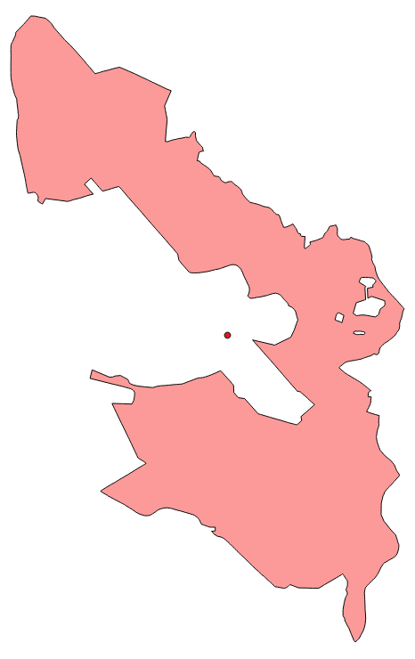
A real-world polygon with a sampling centroid.

Representative point sampling

To deal with this problem, Shapely equips geometry objects with a method called representative_point() that – as the documentation reads – “returns a cheaply computed point that is guaranteed to be within the geometric object”. Judging from the Shapely source code this method goes back to the PointOnSurface function provided by GEOS. I haven’t been able to find out how exactly it is guaranteed that the sample point is an interior point, but from the looks of it, it is most likely that the algorithm described in a fitting thread at gis.stackexchange.com has been applied to it. In any way for our Python example the code would look like the following:

>>> representative_point = polygon.representative_point()
>>> print representative_point
POINT (1.5 3)

Please note that querying for the representative point of a polygon actually calls a Python function – as indicated by the brackets following the according declaration – while the centroid is a property of the Shapely polygon object. Using real-world data we arrive at the situation displayed below:

A real-world polygon with a sampling representative point.

It is also possible to apply the sampler on multi-part polygons:

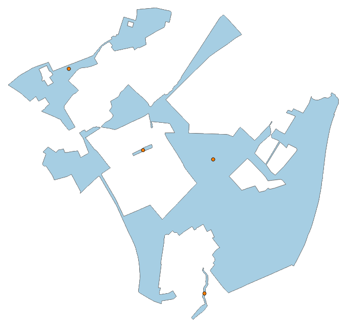
A multi-part polygon consisting of four parts each sampled by a representative point.

Putting it all together

Based on the knowledge laid out above, it is now possible to furnish the previously created PolygonPointSampler base object with extensions that create sample points by either using the centroid or representative point method. I have called them CentroidSampler and RepresentativePointSampler, respectively:

class CentroidSampler(PolygonPointSampler):
    def perform_sampling(self):
        u"""
        Perform sampling by reprensenting each source polygon with its centroid.
        """
        if not self.prepared:
            self.prepare_sampling()
        for src in self.src:
            self.samples.append(src.centroid)
class RepresentativePointSampler(PolygonPointSampler):
    def perform_sampling(self):
        u"""
        Perform sampling by representing each source polygon with a
        representative point whose coordinates are guaranteed to be within
        the polygon's geometry.
        """
        if not self.prepared:
            self.prepare_sampling()
        for src in self.src:
            self.samples.append(src.representative_point())


Creating sample points in a polygon with OGR and Shapely (Introduction)

Creating sample points for a given region of interest is a common task in geospatial analysis. It is therefore logically consistent that there is already a number of ways available to create some including the Create Random Points tool of the ArcToolbox in ArcGIS or the corresponding components of the fTools plugin for QGIS. As I’m trying to follow an explicit under-the-hood-philosophy, I will – starting with this very first “real” entry at Portolan – implement my very own sampling methodology for anyone willing to follow.

As it is my (current) programming language of choice I will use Python to accomplish my task. Adding to the fact that I have plenty of working experience with it, Python has the advantage of being very well positioned in the realm of geospatial processing. This is courtesy of a wide range of libraries dealing with corresponding tasks including two that I will use extensively, namely OGR (as part of GDAL) and Shapely. While OGR serves as a well suited toolbox for all things vector – including export and import to external file and/or database formats, basic dataset creation and editing as well as more sophisticated procedures such as generalization – I have found Shapely (basically representing a Pythonic interface to libgeos that is also used by OGR itself) to be a more direct link to the topological operations that are bread and butter for any kind of geographical information system.

As Python explicitly encourages the object-oriented programming paradigm, I will follow that and implement my very own PolygonPointSampler in compliance to that paradigm. Mind you, I’m not an explicitly stated computer scientist, but a cartographer by trait that somehow turned into a mostly self-taught specialist for geoinformatics. My theoretical ramblings with regard to programming may be a little off from time to time, however all of the things presented here do actually work in practice – which is most important for me. And maybe for the reader as well.

Corresponding to these prerequisites a base class for a PolygonPointSampler could be implemented as set out in the following listing:

u"""
A base class for creating sample points located in a given region of interest,
i.e. polygon.
"""

from shapely.geometry import Polygon

class PolygonPointSampler(object):

    def __init__(self, polygon = ''):
        u"""
        Initialize a new PolygonPointSampler object using the specified polygon
        object (as allocated by Shapely). If no polygon is given a new empty
        one is created and set as the base polygon.
        """
        if polygon:
            self.polygon = polygon
        else:
            self.polygon = Polygon()
        self.samples = list()
        self.sample_count = 0
        self.prepared = False

    def add_polygon(self, polygon):
        u"""
        Add another polygon entity to the base polygon by geometrically unifying
        it with the current one.
        """
        self.polygon = self.polygon.union(polygon)
        self.prepared = False

    def print_samples(self):
        u"""
        Print all sample points using their WKT representation.
        """
        for sample_pt in self.samples:
            print sample_pt

    def prepare_sampling(self):
        u"""
        Prepare the actual sampling procedure by splitting up the specified base
        polygon (that may consist of multiple simple polygons) and appending its
        compartments to a dedicated list.
        """
        self.src = list()
        if hasattr(self.polygon, 'geoms'):
            for py in self.polygon:
                self.src.append(py)
        else:
            self.src.append(self.polygon)
        self.prepared = True

    def perform_sampling(self):
        u"""
        Create a stub for the actual sampling procedure.
        """
        raise NotImplementedError