Monthly Archives: June 2015

Creating sample points (Pt. 3): Uniform random sampling – Triangulation

The third edition of this series will introduce a more complex sampling method to create points that are spread both randomly and uniformly over the area of a given source polygon.

Previously published parts of this series include:

Uniform random sampling

To distribute points in a polygon in a uniform and random manner we are going to follow an approach laid out within the scope of a discussion amongst MATLAB users. In case the internet will forget this minor thread someday, here’s the reduction of the problem as laid out by merited forum contributor John D’Errico:

“[…] the general approach […] that generates uniform random points inside a general object in n-dimensions.

“Compute the area/volume of each simplex, then assign points to them randomly with probability defined by their area relative to the total area. Within each simplex, […] use a […] method of generating random points […].

“Of course, you need a triangulation of the polygon, but as long as the polygon is a convex one, this is trivial with [D]elaunay.”

To summarize these are steps necessary to create uniform random points in a polygon:

  1. Use the polygon’s vertices to create a Delaunay triangulation. As we can’t guarantee that real-world data will only contain convex geometries, this needs to be generalized form of it, a constrained Delaunay triangulation.
  2. Use the area of each created triangle to create a weighted random selection, i.e. to assure that larger triangles a picked more likely than smaller ones.
  3. Randomly create a point inside the selected triangle.

Now these procedure shall be repeated until a certain stop criterion is fulfilled, something that we will discuss later on. Let’s start with triangualation first.

Delaunay triangulation and constrained Delaunay triangulation

Whilst the original (C++) OGR library contains a method DelaunayTriangulation to retrieve just that for an input geometry, this function is not part of the OGR Python bindings. However, as with most tasks there is already another library that can do what we want. In this case we refer to poly2tri. Originally provided in Java and C++, there also exists a Python version of it. (There are some peculiar patches necessary to get poly2tri to work under Python that I will devote another blog entry for.)

Using Shapely and poly2tri it is now possible to initiate a constrained Delaunay triangulation (CDT):

>>> # creating a source polygon first
>>> from shapely.geometry import Polygon
>>> from shapely.wkt import loads
>>> polygon = loads(open(r"real_world_data.wkt").read())
>>> # preparing list of vertices and adding those of current polygon to it
>>> vertices = list()
>>> for coord_pair in polygon.exterior.coords:
...     vertices.append(coord_pair)
>>> # p2t is the Python module name for poly2tri
>>> import p2t

Now two things have to be considered. First, poly2tri brings its very own Point definition that needs to be distinguished from the one Shapely provides by explicitly using the prefix p2t. Adding to that it must be avoided that the CDT is fed with duplicate points – i.e. as first and last vertex are usually specified in polygon definition. We can deal with this constraint by omitting the first vertex:

>>> # making sure that only one of first or last vertex
>>> # is used to create list of input points for triangulation
>>> border = [p2t.Point(x, y) for x, y in vertices[1:]]
>>> # setting up constrained Delaunay triangulation
>>> cdt = p2t.CDT(border)

Now real-world data kicks in back again as it may contain holes, or interior rings as they are called correctly. These need to be specified separately as input for the CDT:

>>> for interior_ring in polygon.interiors:
...     hole = list()
...     for coord_pair in interior_ring.coords:
...             hole.append(coord_pair)
...     else:
...             cdt.add_hole([p2t.Point(x, y) for x, y in hole[1:]])

Finally, the triangulation can be performed:

>>> triangulation = cdt.triangulate()
>>> print len(triangulation)
1964
>>> for t in triangulation:
...     triangle = Polygon([(t.a.x, t.a.y), (t.b.x, t.b.y), (t.c.x, t.c.y)])
...     print triangle
...
POLYGON ((366392.3774440361 5640960.820684713, 367546.1057238859 5641233.076879927, 366393.6058517902 5641064.830985503, 366392.3774440361 5640960.820684713))
POLYGON ((366393.6058517902 5641064.830985503, 367546.1057238859 5641233.076879927, 367452.1526190441 5641333.95416048, 366393.6058517902 5641064.830985503))
...
...

Following is the visual result of the triangulation.

A constrained Delaunay triangulation was applied to this real-world polygon.

Next up in line to create uniformly random sample points are weighted random selection of triangles and random generation of points inside such a given triangle.

Creating sample points (Pt. 2): Regular grid sampling

In this edition of our series dedicated to polygon sampling techniques we will look into the process of creating regularly gridded sample points with non-uniform intervals.

Previously published parts of this series include:

Regular grid sampling

Using a single point to represent a whole polygon geometry may satisfy only the most basic sampling demands. Another – and certainly more applicable – way to arrange sample points is to create virtual grids of such points that stretch out over the whole area of the polygon to be processed. To do so we need a regular interval between sample points that may be defined identical (i.e. uniform) in both x- and y-direction. Here we will go the more generic route and implement separately adjustable (i.e. non-uniform) intervals for x and y.

The value range of sample coordinates is of course laid out by the extent of the source polygon. Using Shapely the extent of a polygon is called forth by the property bounds:

>>> from shapely.geometry import Polygon
>>> polygon = Polygon([(0,0), (6,0), (0,6)])
>>> print polygon.bounds
(0.0, 0.0, 6.0, 6.0)

Given two intervals in x and y it is now easy to create points at regular gridded positions laid out over the extent of the source polygon. Additionally it should be assured that created points are actually within the polygon to be sampled.

>>> from shapely.geometry import Point
>>> bounds = polygon.bounds
>>> ll = bounds[:2] # lower left coordinate pair of polygon's extent
>>> ur = bounds[2:] # upper right                  ~
>>> x_interval = 1.5
>>> y_interval = 2.0
>>> for x in floatrange(ll[0], ur[0], x_interval):
...     for y in floatrange(ll[1], ur[1], y_interval):
...             point = Point(x, y)
...             if point.within(polygon):
...                     print point
...
POINT (1.5 2)
POINT (1.5 4)
POINT (3 2)

Now real-world spatial data is different yet again as it rarely comes with extents fitting to full meters. It is still possible to have regularly gridded sample points that have *nicely* looking coordinates by creating extent ceilings and floors used as base for the sampling process. We can actually use our defined intervals to create these values:

>>> from shapely.wkt import loads
>>> polygon = loads(open(r"real_world_data.wkt").read())
>>> polygon.bounds
(366392.3774440361, 5630693.4900143575, 373404.5164361303, 5641855.842006282)
>>> ll = polygon.bounds[:2]
>>> ur = polygon.bounds[2:]
>>> x_interval = 100
>>> y_interval = 200
>>> low_x = int(ll[0]) / x_interval * x_interval
>>> upp_x = int(ur[0]) / x_interval * x_interval + x_interval
>>> low_y = int(ll[1]) / y_interval * y_interval
>>> upp_y = int(ur[1]) / y_interval * y_interval + y_interval
>>> print low_x, upp_x, low_y, upp_y
366300 373500 5630600 5642000

Putting it all together

To extend our previously introduced PolygonPointSampler, we can combine all our findings in a new sub class RegularGridSampler. This one will also make use of the possibility of creating a separate constructor as there is the need to define the sampling intervals.

class RegularGridSampler(PolygonPointSampler):
    def __init__(self, polygon = '', x_interval = 100, y_interval = 100):
        super(self.__class__, self).__init__(polygon)
        self.x_interval = x_interval
        self.y_interval = y_interval
    
    def perform_sampling(self):
        u"""
        Perform sampling by substituting the polygon with a regular grid of
        sample points within it. The distance between the sample points is
        given by x_interval and y_interval.
        """
        if not self.prepared:
            self.prepare_sampling()
        ll = self.polygon.bounds[:2]
        ur = self.polygon.bounds[2:]
        low_x = int(ll[0]) / self.x_interval * self.x_interval
        upp_x = int(ur[0]) / self.x_interval * self.x_interval + self.x_interval
        low_y = int(ll[1]) / self.y_interval * self.y_interval
        upp_y = int(ur[1]) / self.y_interval * self.y_interval + self.y_interval
        
        for x in floatrange(low_x, upp_x, self.x_interval):
            for y in floatrange(low_y, upp_y, self.y_interval):
                p = Point(x, y)
                if p.within(self.polygon):
                    self.samples.append(p)

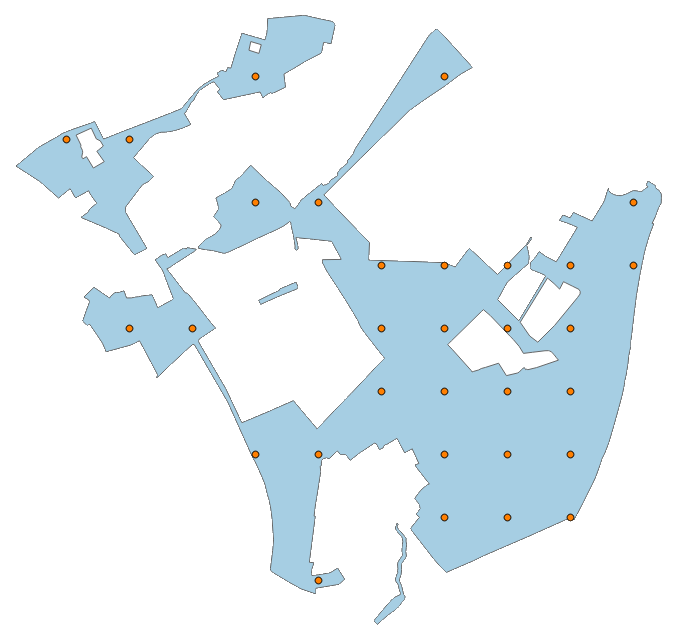
Using our real-world example and a (uniform) sampling interval of 1,000 meters we arrive at the following result:

A real-world polygon with a regular grid of sampling points.

We may also use non-uniform sampling intervals of 1,000 meters in x- and 500 meters in y-direction:

A real-world polygon with a regular grid of sampling points using non-uniform sampling intervals.

A multi-part polygon may also be used to apply the sampler, for example with a uniform sampling interval of 250 m:

A multi-part polygon consisting of four parts sampled by a regular grid with a uniform sampling interval of 250 m.

WTH is a floatrange?

In the meantime you most likely have already realized that we’re using a non-standard range function to iterate over a range of float values. Based on a StackExchange suggestion I have defined an according routine in a utility function:

def floatrange(start, stop, step):
    while start < stop:
        yield start
        start += step